Thermohaline Circulation - Exploration

Your Objective

How does the atmosphere influence the ocean to drive large-scale vertical circulation (ocean conveyor)?

Explore the data below to see what you can observe.
Make a prediction about how the SST (using 30 m depth as a proxy for the surface) responds to seasonal changes in wind forcing.
Make a prediction about how the ocean surface water density changes in response to changes in the wind forcing.
Make a prediction about how the surface water moves in response to changes in its density.

Specify temperatures to plot:

30m Model Air Temperature

Data Tips

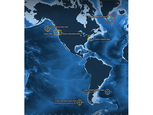
When the site loads, you are able to see the full dataset of wind speed, seawater temperature, and seawater density for the POR of 2014-09-21 to 2018-06-17 from the Irminger Sea Flanking Mooring B and ECMWF reanalysis grid point. You can interact with the data by:

Turning on and off the various layers of temperature, density, and speed. If a reference layer is needed, I suggest the ECMWF wind speed OR the 30m temperature.
Zoom in and out of the data to highlight particular sections of the seasonal cycle. Site loads with all data highlighted, change highlighted width with zoom.

Questions for Thought

Orientation Questions

What oceanic and atmospheric variables are displayed in the graphs? What are the units associated with each variable?
What time period does the graph cover?
- What is the starting date?
- What is the ending date?
- How many complete years of data are represented?
What graph type is this?

Interpretation Questions

What changes or patterns did you observe in the surface temperature graph?
Does this change correlate with the surface wind speed data?
What is the relationship between ocean water temperature and ocean water density?
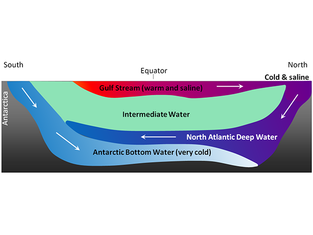
What does the seasonal change in surface density imply about the initiation of the thermohaline circulation at the Irminger Sea area?

Background Information

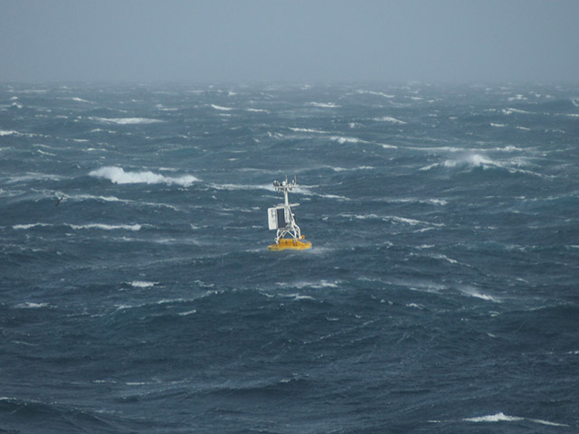
Click on the images below to learn more about where and how the dataset above was collected.

Dataset Information

The data for this activity was obtained from the following CTDs on the Irminger Sea Flanking Mooring B:

Recovered datasets were downloaded from the OOI data portal, and then daily (mean) averages of temperature and density were calculated and merged together into a single file. Potential temperature and potential density were calculated using the seawater toolbox.

Because the meteorological data from the Irminger Surface Mooring is rather sparse, wind speed and air temperature data was obtained from the ECMWF reanalysis at the closest grid points (between 59-61°N and 40-38°W).

The highlighted boxes represent those time periods where the difference between the 350m and 30m potential density is less than 0.05 kg/m³. This effectively highlights those time periods when the mixed layer depth reaches far below the surface.

See this Jupyter Notebook for details on how the data for this activity was processed.

Activity Citation: Dixon, R., Beaird, N., & Lichtenwalner, C. S. (2019). Thermohaline Circulation. OOI Data Labs Collection.